Introduction to image processing using Python
Posted on Monday, 19 April 2021.
Basic image processing tools may serve you in many situations as a developer, and there are several libraries to help you with image processing tasks (this statement is particularly true if you are a Pythonist). However, knowing how to implement basic procedures is not only a good programming exercise but will give you the ability to tweak things to your liking. In this article, we will see how to implement basic image processing tools from scratch using Python.
Requirements
Besides Python 3 you will need:
Imageio: To read and write images. Installation:
$ pip install imageio
Numpy: Used to store and manipulate arrays. Installation:
$ pip install numpy
Matplotlib: Used to plot the simplified RGB space. Installation:
$ pip install matplotlib
tqdm: Used to generate progress bars. Installation:
$ pip install tqdm
Toolbox
Our basic image processing toolbox will consist of:
| Tool | Effect |
|---|---|
| Grayscale | Converts an RGB image into grayscale using the luminance of a pixel. |
| Halftone | Converts the range of a grayscale image to $[0, 9]$, i.e. $10$ shades of gray, and for each pixel value performs a mapping, such that the output is a black and white picture that resembles a grayscale picture with lower resolution. |
| Mean blur | Takes an average of $3 \times 3$ regions. |
| Gaussian blur | Takes a weighted average of a $3 \times 3$ region using a gaussian function. |
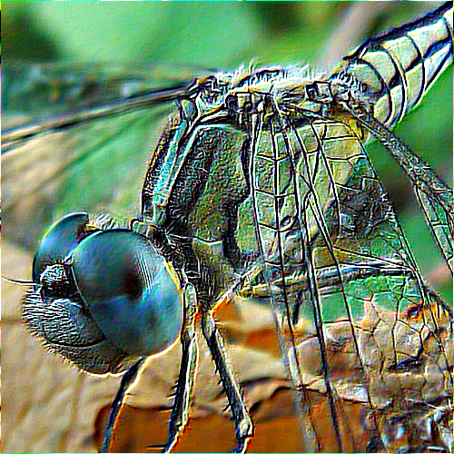
| Sharpen | Sharpens the image. Formally, it substracts the 4-neighbors laplacian from the original image. |
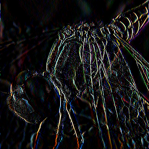
| Laplacian | Returns the $8-$neighbors laplacian applied to the image. |
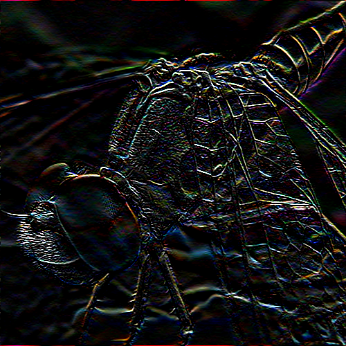
| Emboss | Enhance image emboss. |
| Motion blur | Blurs the image as if the camera (or object) is moving. |
| Edge detectors | Sobel filters to detect vertical and horizontal edges, respectively. |
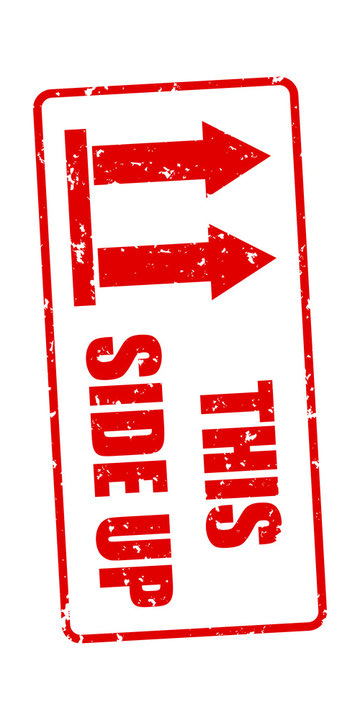
| $90^{\circ}$ rotation | Rotates the image $90^{\circ}$ clockwise. |
| $180^{\circ}$ rotation | Rotates the image $180^{\circ}$. |
| $-90^{\circ}$ rotation | Rotates the image $90^{\circ}$ counterclockwise. |
| Flips | Vertical and horizontal flips. |
| Intensity | Brightens or darkens the image. |
| Negative | Produces the negative of an image. |
Basic Concepts
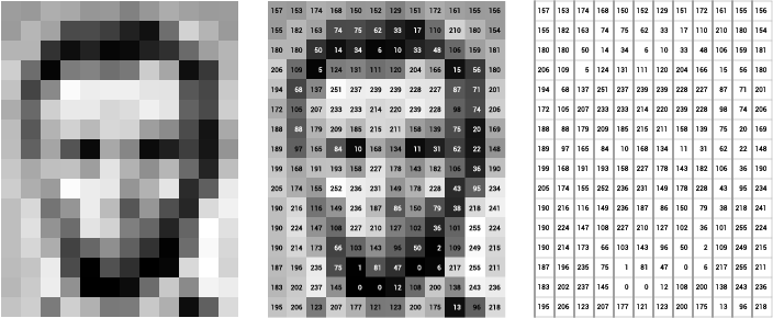
In a nutshell, digital cameras have a bidimensional array of sensors to record values proportional to the intensity of the light hitting that sensor in a given position (pixel). The digital image is then stored as a bidimensional array whose values (in a given scale) represent the intensity of light in that pixel position, as shown in the figure below.
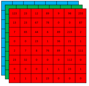
For RGB images this process is very similar, the only difference being that we need three of such bidimensional arrays stacked to compose the image. The actual manner we combine the sensor data (bidimensional) to obtain RGB images (with an extra dimension representing the color channels) is a subject of its own and we will not deal with this problem here.
The range of values allowed may vary. However, the two most common representations are $8-$bit integer images (discrete values in $[0, 255]$) and images whose pixels values are float numbers in $[0, 1]$.
As we will see, any image processing tool is simply a manipulation of these pixel values, either changing the actual value or its position in the array.
Grayscale Images
There are many ways to convert RGB images into grayscale images. For instance, in the RGB representation, if the intensity values of the three channels in a pixel are the same, then the result color is a shade of gray. As you can see in the figure below, the diagonal of the RGB space, i.e. when $R=G=B$, is a grayscale line with black corresponding to $R=G=B=0$ and white corresponding to $R=G=B=1$ (or $255$).
import numpy as np
import matplotlib.pyplot as plt
from mpl_toolkits import mplot3d

fig = plt.figure()
ax = plt.axes(projection="3d")

t = np.linspace(0, 1, 1000, endpoint=True)
for i in t:
    ax.scatter3D(i, i, i, color=(i,i,i))
    ax.scatter3D(i, 0, 0, color=(i,0,0))
    ax.scatter3D(0, i, 0, color=(0,i,0))
    ax.scatter3D(0, 0, i, color=(0,0,i))
plt.show()
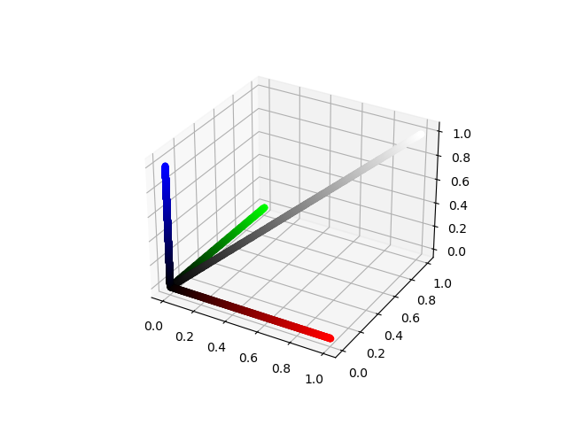
One could therefore convert a colored image into a grayscale image by assigning the pixel value to have the average of the intensities in the red, green, and blue channels. In this article, however, we will use the luminance of a pixel to do this task. The luminance of a pixel is defined to be $$Y \equiv 0.299r + 0.587g + 0.114b, $$ where $r$, $g$, and $b$ are the red, green, and blue pixel values of the image. Therefore, to convert our RGB image into grayscale, we need to assign the new pixel value to the corresponding luminance value of that pixel. Let us build our first image processing tool, the grayscale converter.
import imageio
import numpy as np
from tqdm import tqdm

def get_shape(image):
    shape = image.shape
    if len(shape)==3 or len(shape)==2:
        return shape
    else:
        raise Exception("Sorry, something is wrong!")

def is_grayscale(image):
    if len(get_shape(image))==3:
        return False
    elif len(get_shape(image))==2:
        return True
    else:
        raise Exception("Sorry, something is wrong!")

def get_luminance(image):
    return 0.299*image[:, :, 0] + 0.587*image[:, :, 1] + 0.114*image[:, :, 2]

def zeros(height, width, depth=None):
    return np.zeros((height, width)) if depth is None else np.zeros((height, width, depth))

def convert_grayscale(image):
    if not is_grayscale(image):
        height, width, _ = get_shape(image)
        gray_image       = zeros(height, width)
        gray_image = get_luminance(image)
        return gray_image
    else:
        return image
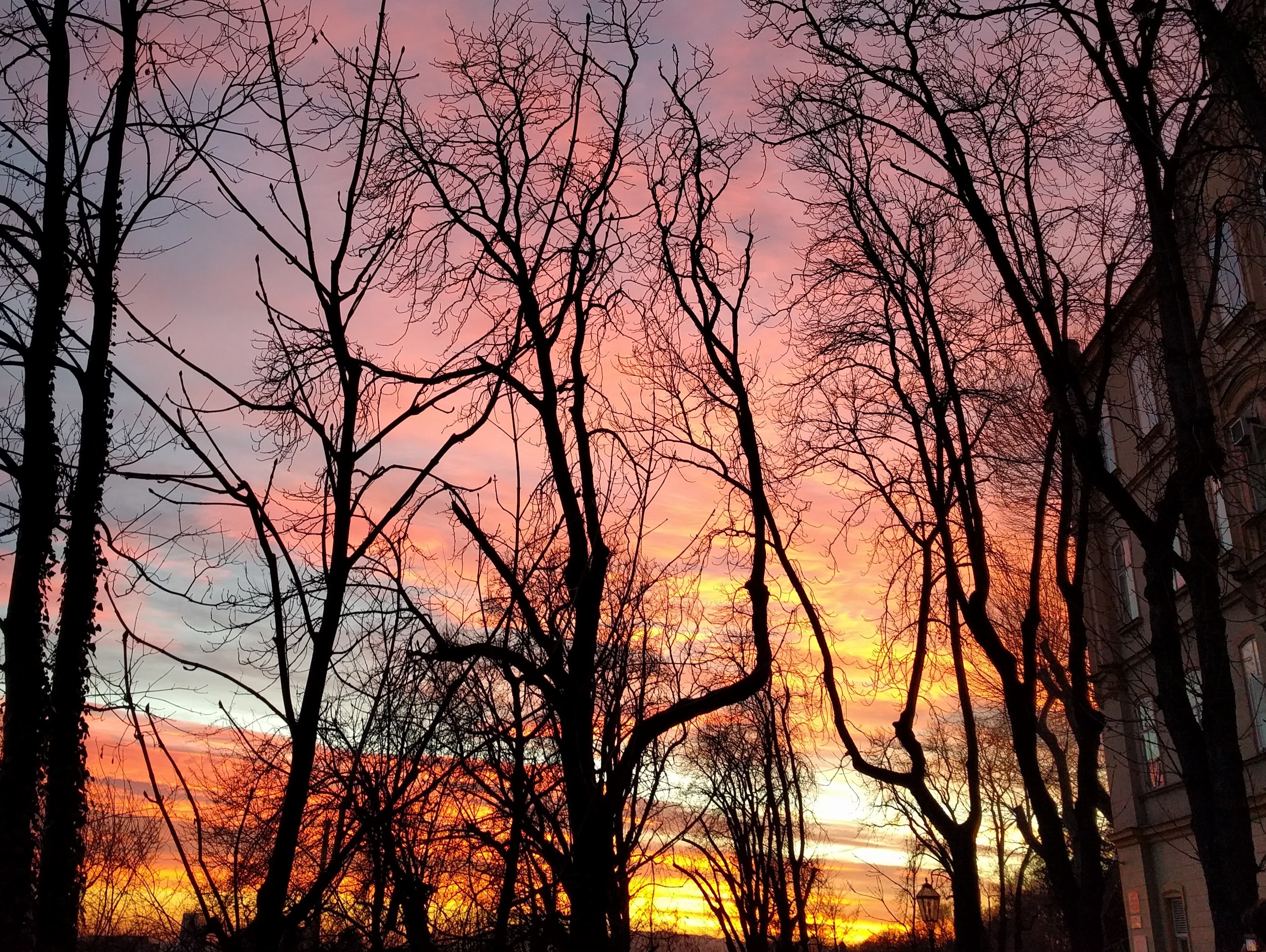
Let us apply to a picture and see the result:
path = "zagreb.jpg"
image = imageio.imread(path)
gray = convert_grayscale(image).astype(np.uint8)
imageio.imwrite("zagreb_grayscale.png", gray)
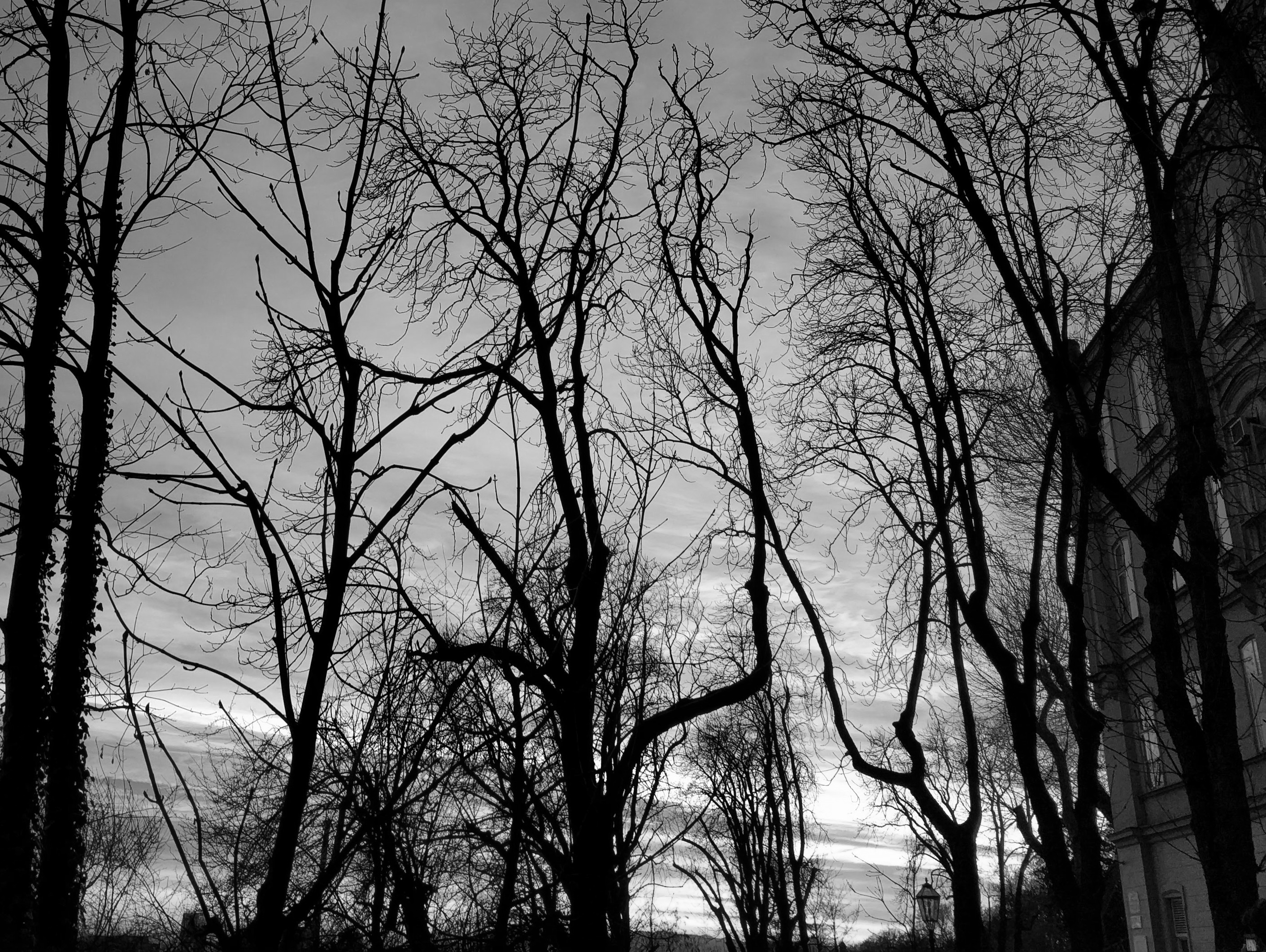
Cool! We have built a grayscale image converter from scratch. Let’s use it to generate a halftone image.
Halftone Images
Halftone is a technique to approximate shades of gray using dot patterns. Here, we want to use $10$ shades of gray, thus each gray level will be represented by a $3\times 3$ pattern of black and white dots. To generate our halftone image, we need to rescale the pixel intensities to the discrete range $[0 , 9]$ and apply the mapping given in the figure below.
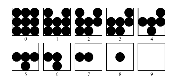
The formula to rescale the pixel values to a given range is given by
\begin{eqnarray*} \hat{I}(x,y) = &\lambda& * (I(x,y) - \min(I(x,y)))\newline &+& \text{newMin} \end{eqnarray*} with $$\lambda = \frac{\text{newMax} - \text{newMin}}{ \max(I(x,y)) - \min(I(x,y)) },$$
$I(x, y)$ representing the original image, and $\hat{I}(x,y)$ representing the image in the new range. These steps are summarized in the piece of code below.
# Add this code after the grayscale converter

def get_image_range(image):
  return np.min(image), np.max(image)

def adjust_gray(image, new_min, new_max):
  image_min, image_max = get_image_range(image)
  h, w  = get_shape(image)
  adjusted = zeros(h, w)
  adjusted = (image - image_min)*((new_max - new_min)/(image_max - image_min)) + new_min
  return adjusted.astype(np.uint8)

def gen_halftone_masks():
  m = zeros(3, 3, 10)

  m[:, :, 1] = m[:, :, 0]
  m[0, 1, 1] = 1

  m[:, :, 2] = m[:, :, 1]
  m[2, 2, 2] = 1

  m[:, :, 3] = m[:, :, 2]
  m[0, 0, 3] = 1

  m[:, :, 4] = m[:, :, 3]
  m[2, 0, 4] = 1

  m[:, :, 5] = m[:, :, 4]
  m[0, 2, 5] = 1

  m[:, :, 6] = m[:, :, 5]
  m[1, 2, 6] = 1

  m[:, :, 7] = m[:, :, 6]
  m[2, 1, 7] = 1

  m[:, :, 8] = m[:, :, 7]
  m[1, 0, 8] = 1

  m[:, :, 9] = m[:, :, 8]
  m[1, 1, 9] = 1

  return m

def halftone(image):
  gray      = convert_grayscale(image)
  adjusted  = adjust_gray(gray, 0, 9)
  m         = gen_halftone_masks()

  height, width = get_shape(image)
  halftoned        = zeros(3*height, 3*width)
  for j in tqdm(range(height), desc = "halftone"):
      for i in range(width):
          index = adjusted[j, i]
          halftoned[3*j:3+3*j, 3*i:3+3*i] = m[:, :, index]

  halftoned = 255*halftoned
  return halftoned
Time to test it!
path = "test.png"
image = imageio.imread(path)
ht = halftone(image).astype(np.uint8)
imageio.imwrite("halftone.png", ht)

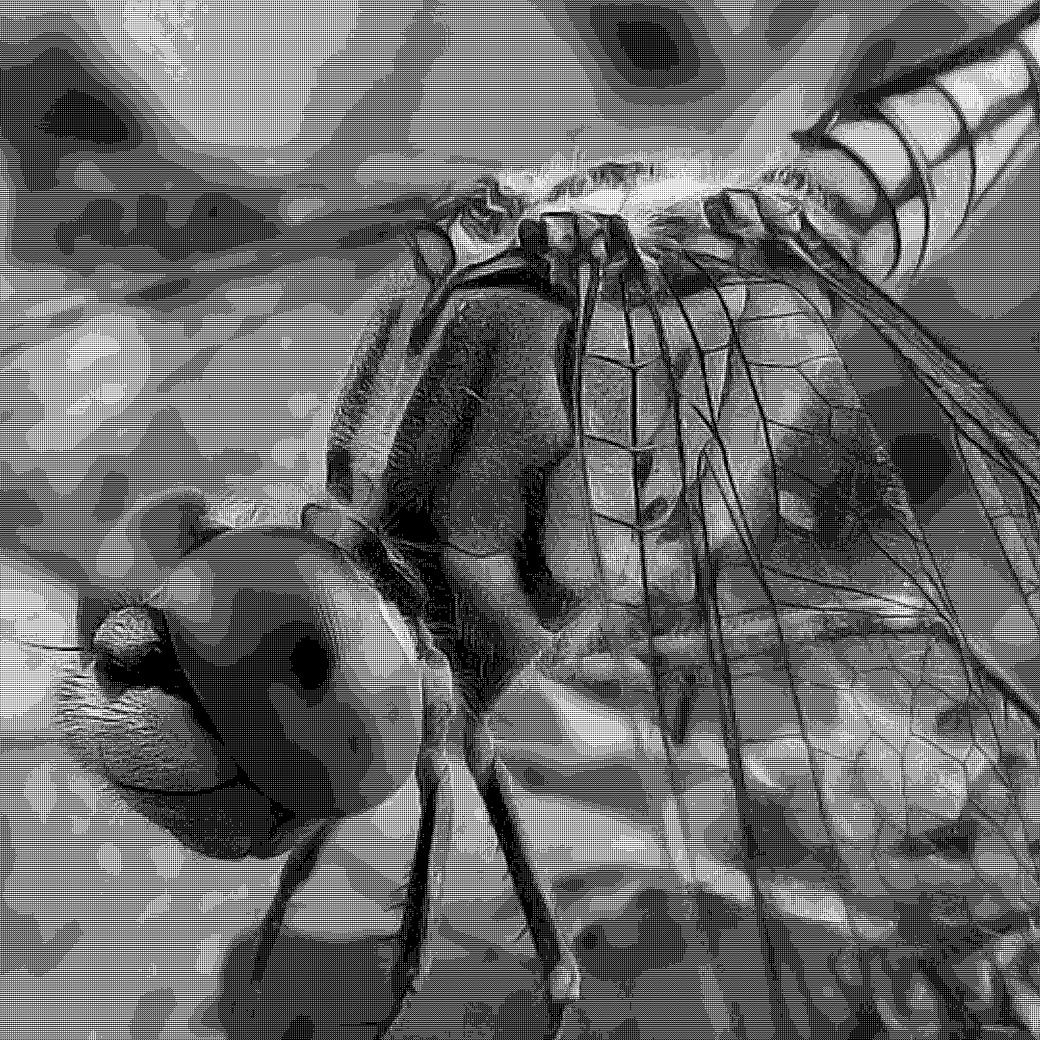
Remember, the image on the right-hand side is a black and white (binary) picture using the dot pattern above. How amazing is that? This technique was broadly used to print photographs in newspapers to simulate shades o grays.
Cross-Correlation and Filters
Arguably, the most popularized concept used in image processing is the one of a convolution. It has been used, successfully, in many Deep Learning architectures and popularized by the so-called Convolutional Neural Networks. Notwithstanding, what people call convolution in this context is actually formally called cross-correlation or spatial correlation. But what is it and how to implement it?
Mathematically, the cross-correlation of a kernel $\omega$ of size $m \times n$ with an image $f(x,y)$ of size $M \times N$ is given by
$$(\omega \ast f)(x,y) = {\sum_{s=-a}^{a}}{\sum_{t=-b}^{b}}\omega(s,t)f(x+s, y+t).$$
Note that the center coefficient of the kernel, $\omega(0,0)$ , aligns with the pixel at location $( x , y )$, visiting it exactly once. For a kernel of size $m \times n$ , we assume that $m = 2 a + 1$ and $n = 2 b + 1$, where $a$ and $b$ are nonnegative integers. This means that our focus is on kernels of odd size in both coordinate directions.
In English, one should “slide” the kernel $\omega$ through the image, evaluating the sum of the pixelwise product between the kernel and the corresponding region of the image, and assign that value to the current pixel location (the center of the kernel, in our case). This general idea is depicted in the animation below.
I encourage you to research the differences between convolution and the correlation defined here. However, there is a certain equivalence between these two operations.
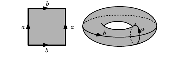
When dealing with convolution/cross-correlation, it is important to pay attention to the edges of the image. There are boundary conditions one could implement, such as zero paddings, or repeating the same values found in the edges of the image. I also encourage you to implement them by yourself. In this article, however, we are going to implement the periodic, or wrapped, boundary condition. Briefly, whenever the filter crosses one edge, it comes through the opposite boundary, just like a Pacman game or a torus.
Ok, no more math. The final code consists of a dictionary containing all of our kernels and the apply_kernel function, a.k.a the cross-correlation. If the image has three channels, we apply the cross-correlation in each channel and combine the results. Take a look at the description box at the beginning of this article, the definition of cross-correlation, and the corresponding kernels. Can you figure out why they work?
# Add this after your halftone method

def clip(a):
    return np.clip(a, 0, 255)

kernels = {"mean"      : np.array([[1/9, 1/9, 1/9],
                                   [1/9, 1/9, 1/9],
                                   [1/9, 1/9, 1/9]]),

           "gaussian"  : np.array([[1/16, 2/16, 1/16],
                                   [2/16, 4/16, 2/16],
                                   [1/16, 2/16, 1/16]]),

           "sharpen"   : np.array([[0 , -1,  0],
                                   [-1,  5, -1],
                                   [0 , -1,  0]]),

           "laplacian" : np.array([[-1, -1, -1],
                                   [-1,  8, -1],
                                   [-1, -1, -1]]),

           "emboss"    : np.array([[-2, -1, 0],
                                   [-1,  1, 1],
                                   [ 0,  1, 2]]),

           "motion"    : np.array([[1/9, 0, 0, 0, 0, 0, 0, 0, 0],
                                   [0, 1/9, 0, 0, 0, 0, 0, 0, 0],
                                   [0, 0, 1/9, 0, 0, 0, 0, 0, 0],
                                   [0, 0, 0, 1/9, 0, 0, 0, 0, 0],
                                   [0, 0, 0, 0, 1/9, 0, 0, 0, 0],
                                   [0, 0, 0, 0, 0, 1/9, 0, 0, 0],
                                   [0, 0, 0, 0, 0, 0, 1/9, 0, 0],
                                   [0, 0, 0, 0, 0, 0, 0, 1/9, 0],
                                   [0, 0, 0, 0, 0, 0, 0, 0, 1/9]]),

           "y_edge"    : np.array([[1 ,  2, 1],
                                   [0 ,  0, 0],
                                   [-1, -2,-1]]),

           "x_edge"    : np.array([[1, 0, -1],
                                   [2, 0, -2],
                                   [1, 0, -1]]),

            "identity" : np.array([[0, 0, 0],
                                   [0, 1, 0],
                                   [0, 0, 0]])}

def apply_kernel(image, kernel):
    kernel_matrix = kernels.get(kernel)
    dim           = len(kernel_matrix)
    center        = (dim - 1)//2

    shape = get_shape(image)
    height, width = shape[0], shape[1]

    if not is_grayscale(image):
        picture = zeros(height, width, 3)

        for y in tqdm(range(height), desc = kernel):
            for x in range(width):

                red = zeros(dim, dim)
                for i in range(dim):
                    for j in range(dim):
                        red[i , j] = image[ (y - center + j)%height, (x - center + i)%width, 0]

                green = zeros(dim, dim)
                for i in range(dim):
                    for j in range(dim):
                        green[i , j] = image[ (y - center + j)%height, (x - center + i)%width, 1]

                blue = zeros(dim, dim)
                for i in range(dim):
                    for j in range(dim):
                        blue[i , j] = image[ (y - center + j)%height, (x - center + i)%width, 2]

                redc   = np.sum(red*kernel_matrix)
                greenc = np.sum(green*kernel_matrix)
                bluec  = np.sum(blue*kernel_matrix)

                r, g, b = map(int,  [redc, greenc, bluec])
                r, g, b = map(clip, [r, g, b])

                picture[y, x, 0] = r
                picture[y, x, 1] = g
                picture[y, x, 2] = b
        return picture
    else:
        picture = zeros(height, width)
        for y in tqdm(range(height), desc = kernel):
            for x in range(width):

                aux = zeros(dim, dim)
                for i in range(dim):
                    for j in range(dim):
                        aux[i , j] = image[ (y - center + j)%height, (x - center + i)%width]
                gray = np.sum(aux*kernel_matrix)

                pxl_intensity = round(gray)
                pxl_intensity = clip(pxl_intensity)
                picture[y, x] = int(pxl_intensity)
        return picture
Finally,
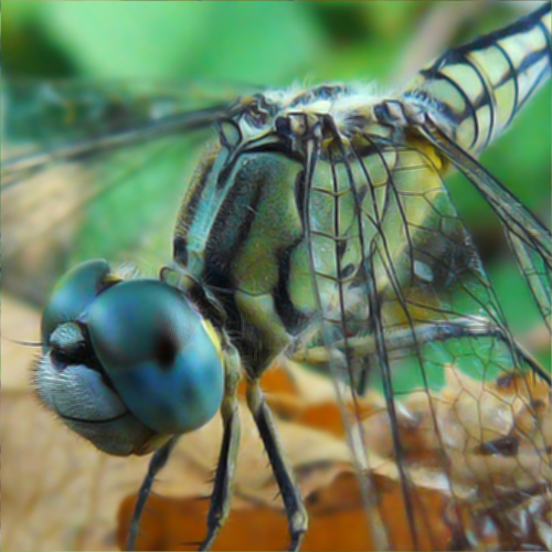
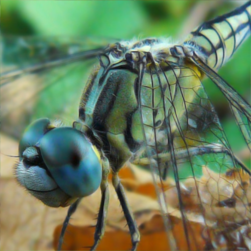
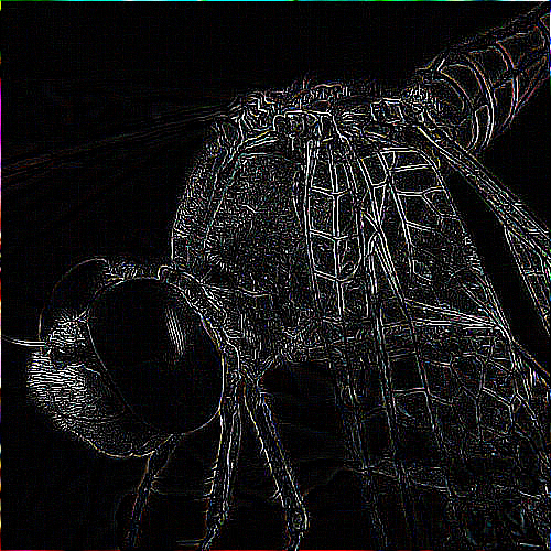
path = "test.png"
image = imageio.imread(path)
for key in kernels:
    img = apply_kernel(image, key).astype(np.uint8)
    imageio.imwrite(key + ".png", img)
The results are given in the mosaic below (in a row-major manner).


Geometric Transformations
Let us now see some geometric transformations. These are transformations that change the order of the pixels, not their actual values. Here we include multiples of $90^{\circ}$ rotations and flips along the vertical and horizontal axes. For more general rotations and flips we need to use some form of interpolation and, for the sake of simplicity, we will avoid them here. The main ingredient here is the slice notation used in Python, so if you are not familiar with it that is a great use case for it!
Rotations
First, let us see the case of a $90^{\circ}$ rotation. In terms of matrices, we can think of a $90^{\circ}$ rotation as the composition of two simple operations. First, we transpose the matrix, then we rearrange the columns in the reverse order (try it with a $2 \times 2$ matrix). For a $180^{\circ}$ rotation we can reverse the order of the rows and columns. Finally, for a $-90^{\circ} = 270^{\circ}$ rotation we can apply the $180^{\circ}$ and $90^{\circ}$ together.
Flips
Flips along the vertical or horizontal axis are very simple operations. A vertical flip is obtained by reversing the rows, whereas a horizontal flip is obtained by reversing the columns. Simple as that!

Our Python code for geometric transformations is:
def transpose(m):
    height, width, depth = get_shape(m)

    transposed = zeros(width, height, depth)
    for i in range(width):
        for j in range(height):
            transposed[i, j] = m[j, i]
    return transposed

def aux90(image):
    return transpose(image)[:,::-1]

def rot90(image):
    print("Rotating the image 90 degrees clockwise...")
    rot = aux90(image)
    return transpose(image)[:,::-1]

def rot180(image):
    print("Rotating the image 180 degrees...")
    rot = image[::-1, ::-1]
    return rot

def rotm90(image):
    print("Rotating the image 90 degrees counterclockwise...")
    rot = aux90(image[::-1, ::-1])
    return rot

def vert_flip(image):
    print("Flipping vertically...")
    flip = image[::-1]
    return flip

def hor_flip(image):
    print("Flipping horizontally...")
    flip = image[:, ::-1]
    return flip
Collecting everything in a dictionary and running the code, we have:
geometric_transforms = {"rot90" : rot90,
"rot180" : rot180,
"rotm90" : rotm90,
"vert_flip" : vert_flip,
"hor_flip" : hor_flip}
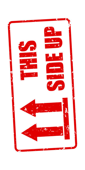
path = "arrows.jpg"
image = imageio.imread(path)
for key in geometric_transforms:
img = geometric_transforms[key](image).astype(np.uint8)
imageio.imwrite(key + ".png", img)


Intensity Transformations
Now, we are going to see how to brighten/darken an image. As we have seen, the pixel values represent, in some scale, the intensity of the light in that position. To brighten or darken an image, all we need is to multiply every value by the same amount $\lambda > 0$. If $\lambda > 1$, the resulting image will be brighter than the original, and if $\lambda < 1$ the resulting image will be darker than the original image. For $\lambda > 1$, some values might exceed the allowable range (e.g, exceed $255$ for $8-$bit images). In that case, we need to clip the result (already implemented). The corresponding Python code is given below.
def intensity(image, factor):
   return clip(factor*image)
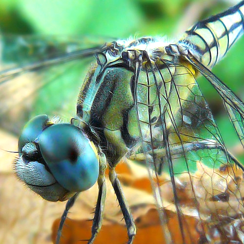
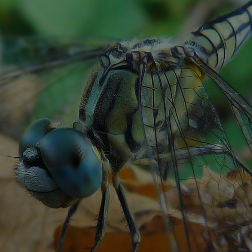
The results of a $25$% increase in brightness and a $50$% decrease in brightness are given below.
path = "test.png"
image = imageio.imread(path)
img_brighter = intensity(image, 1.25).astype(np.uint8)
imageio.imwrite("brighter.png", img_brighter)
img_darker = intensity(image, 0.5).astype(np.uint8)
imageio.imwrite("darker.png", img_darker)
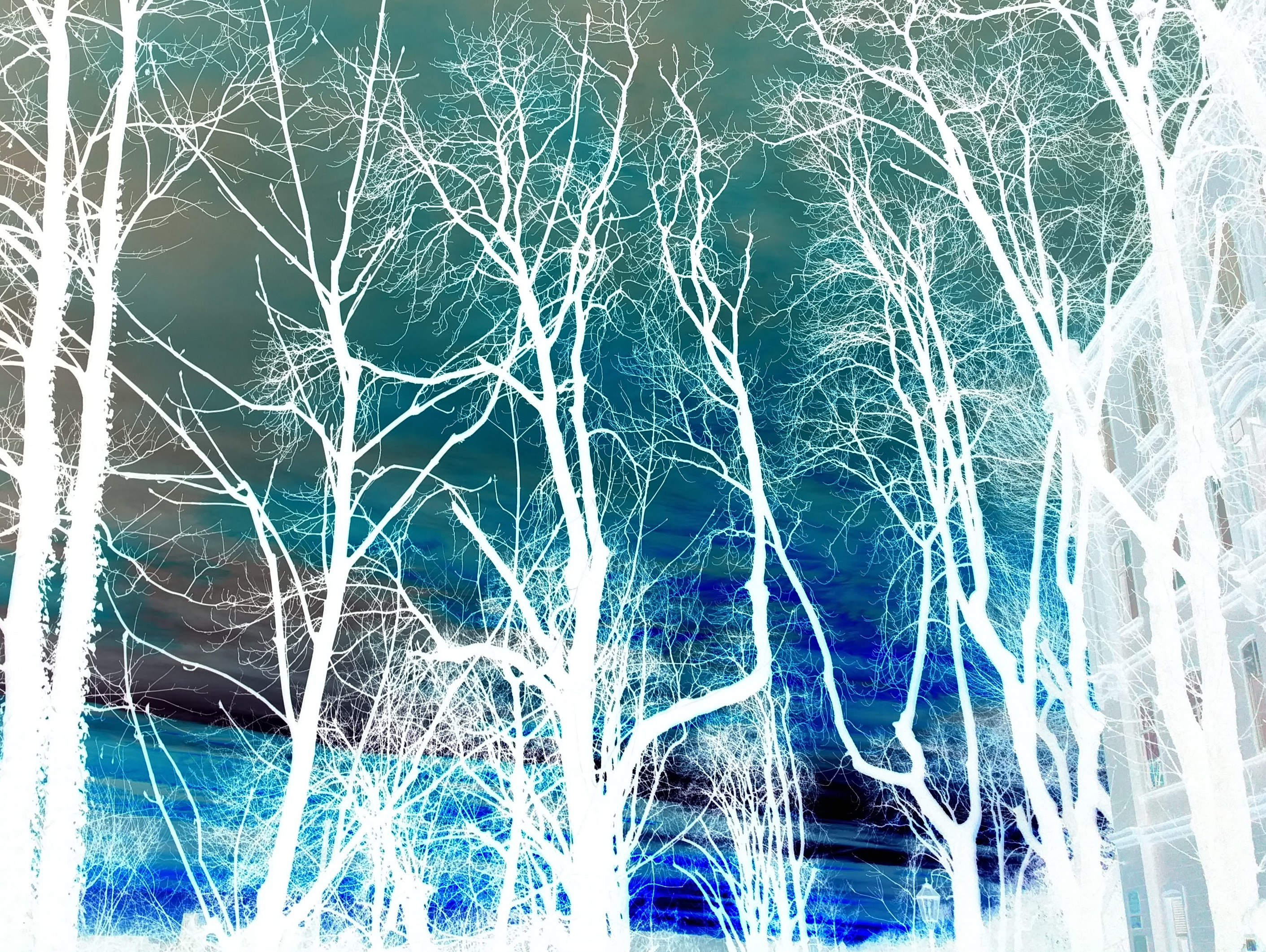
Negative Images
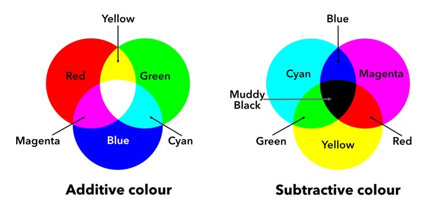
Images represented in the RGB color model consist of three components, one for each primary color. When fed into an RGB monitor, these three images combine on the screen to produce a composite color image. The secondary colors of light are cyan (C), magenta (M), and yellow (Y). They are also known as the primary colors of pigments. For instance, when a surface coated with cyan pigment is illuminated with white light, no red light is reflected from the surface. In a nutshell, cyan is the absence of red, magenta is the absence of green, and yellow is the absence of blue. Because of that, we usually interpret the RGB model to be additive, whereas the CMY is subtractive (see the image below).
“A positive image is a normal image. A negative image is a total inversion, in which light areas appear dark and vice versa. A negative color image is additionally color-reversed, with red areas appearing cyan, greens appearing magenta, and blues appearing yellow, and vice versa.”
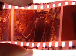
A similar concept is used in negative films if you happen to be old enough to remember what they are.
Now, in terms of implementation, we have a very simple function (thanks to Numpy broadcasting).
def negative(image):
  return 255 - image
As a result:
path = "zagreb.jpg"
image = imageio.imread(path)
img = negative(image).astype(np.uint8)
imageio.imwrite("zagreb_negative.png", img)
Conclusion
Congratulations! You have built your first image processing toolbox! Although we have used a Pythonic way to implement things here and there, you can use the concepts outlined here to implement everything in any other language.
Now that you know how to implement these tools yourself you can use them in your application. Be creative, combine and tweak these tools to your liking. I know you will find many use cases for it! For instance, I have been using some of these implementations for data augmentation purposes in Machine Learning, since they are fairly easy to implement on the fly and prevent you to store several additional images on your computer.
Recommended Reading
By clicking and buying any of these from Amazon after visiting the links above, I might get a commission from their Affiliate program, and you will be contributing to the growth of this blog :)